(L1) Graphical Limits#
By the end of the lesson you will be able to:
find the one-sided limits of a function using graphical methods.
use the one-sided limits to determine the (overall) limit of a function using graphical methods.
Lecture Video#
Reading a Graph#
To begin, we are going to quickly review how we actually read the graph of a function:
Input Values - are read from the horizontal axis. These are what gets plugged into the function.
Output Values - are read from the vertical axis. These are essentially the values that the function returns to us.
When we find a point \((a,b)\) on the graph of a function \(f\). The input value is \(x=a\) and the output value of the function at \(x=a\) is then given by the \(y\)-coordinate of the point. So the output value would be \(f(a)=b\).
Example#
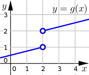
Suppose we are given the graph of function \(y=g(x)\) below. Use this graph to evaluate the following function values.
(a) Evaluate \(g(1)\)
Based on the graph, \(g(1)=0.75\)
To determine this, we find \(x=1\) along the \(x\)-axis, read up to find the corresponding point on the graph which looks to be about \((1,0.75)\).
The \(y\)-coordinate of this point is then the output value of the function at \(x=1\).
(b) Evaluate \(g(4)\)
Based on the graph, \(g(4)=2.5\)
To determine this, we find \(x=4\) along the \(x\)-axis, read up to find the corresponding point on the graph which looks to be about \((4,2.5)\).
The \(y\)-coordinate of this point is then the output value of the function at \(x=4\).
(c) Evaluate \(g(2)\)
Based on the graph, \(g(2)\) is undefined.
Because the two points at \(x=2\) are denoted using open circles, neither of them are actually included in the graph.
Graph Notation#
An Open Circle denotes a point that is not actually included on the graph.
A Filled-in Circle denotes a point that is included on the graph.
One-Sided Limits#
Introduction#
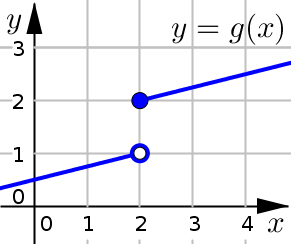
In the graph below, note the interesting behavior around \(x=2\).
What point does the left side of our curve approach near \(x=2\)?
On the left side, it looks like the curve is getting closer and closer to the point \((2,1)\) … even though this point is not actually included in the graph (because it is an open dot).
Because the graph is getting closer to the point \((2,1)\) on this left side we write:
where the limit is equal to the \(y\)-coordinate of the point we are approaching.
What point does the right side of our curve approach near \(x=2\)?
On the right side, it looks like the curve is getting closer and closer to the point \((2,2)\).
Because the graph is getting closer to the point \((2,2)\) on this right side we write:
where the limit is equal to the \(y\)-coordinate of the point we are approaching.
One-Sided Limit Definitions#
As smaller input values, \(x\), get close to the number \(a\), the ouptut values, \(f(x)\), get close to the number \(L\).
Left Side Limit
As larger input values, \(x\), get close to the number \(a\), the ouptut values, \(f(x)\), get close to the number \(L\).
Right Side Limit
You can remember this notation by:
\(a^-\) means we are close to \(a\) but have subtracted a little.
\(a^+\) means we are close to \(a\) but have added a little.
(Overall) Limit#
Definition#
(Overall) Limit of a Function
We say that the number \(L\) is the limit of \(f(x)\) as \(x\) approaches \(a\),
Provided: \(f(x)\) can be made arbitrarily close to \(L\) for all \(x\) sufficiently close (but not equal) to \(a\).
In this case we write: \( \displaystyle \lim_{x\to a} f(x) = L \)
Relationship to One-Sided Limits#
Specifically we write:
provided both of the left and right sided limits are equal to \(L\)
Note: It does not matter what happens directly at \(x=a\), with a limit we are only concerned with what happens as the input values get closer to \(a\) from either side.
Warning
If the left and right limits are not equal to each other we say the overall limit \(\displaystyle \lim_{x\to a} f(x)\) does not exist (DNE).
Example 1#
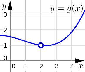
Use the graph to compute \(\displaystyle \lim_{x\to 2} g(x)\)
Solution and Explanation
From the left side we see that the graph is getting closer to the point \((2,1)\). Therefore the left side limit is: \(\displaystyle \lim_{x\to 2^-} g(x)=1\)
From the right side we see that the graph is getting closer to that same point \((2,1)\). Therefore the right side limit is: \(\displaystyle \lim_{x\to 2^+} g(x)=1\)
Since the left and right side limits are equal, the overall limit is \(\displaystyle \lim_{x\to 2} g(x)=1\)
Example 2#
Use the graph to compute \(\displaystyle \lim_{x\to 2} g(x)\)

Solution and Explanation
From the left side we see that the graph is getting closer to the point \((2,1)\). Therefore the left side limit is: \(\displaystyle \lim_{x\to 2^-} g(x)=1\)
From the right side we see that the graph is getting closer to that same point \((2,2)\). Therefore the right side limit is: \(\displaystyle \lim_{x\to 2^+} g(x)=2\)
Since the left and right side limits are not equal, the overall limit \(\displaystyle \lim_{x\to 2} g(x)\) does not exist.
Graphical Issues#
Estimates: The main issue with these graphical and numerical methods for calculating a limit is that they are both technically estimates. They give us a way to estimate the value of a limit (we’ll see how to calculate them exactly using algebraic methods).
False Positive: One of the issues we might encounter is a false positive. This can happen by just choosing unlucky input values to plug-in. As we can see in the graph below, if we had had the misfortune of picking all the \(x\)-values where the function crosses the horizontal axis, we might be tempted to conclude that \(\displaystyle \lim_{x\to0^+} f(x) =0\).
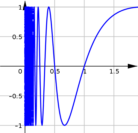
However someone else may have picked all the \(x\)-values where the function has a maximum value of \(1\), and a third person may have picked all the \(x\)-values where the function has its minimum value of \(-1\).
In fact this limit\(\displaystyle \lim_{x\to0^+} f(x)\) does not exist because as \(x\) gets closer to \(0\) from the right, the function bounces back and forth and repeatedly takes on all values between \(-1\) and \(1\).
