(DC5) Graphical Estimations#
By the end of the lesson you will be able to:
graphically estimate the value of the derivative at a point.
interpret the meaning of a derivative in context and state the units.
Lecture Videos#
Interpreting the Derivative#
Since we’ve started exploring the derivative, we have primarily been looking at two examples: tangent lines and velocity. However, the derivative has a significance in many diverse fields, so it will be helpful to generalize some of the terminology:
Difference Quotient
Limit of the Difference Quotient
Tangent Lines - If function \(f\) represents the height of the graph, then the:
difference quotient represents the slope of a secant line.
limit of the difference quotient represents the slope of the tangent line.
Velocity - If function \(f\) represents the position of an object moving in a straight line, then the:
difference quotient represents the average velocity over a time interval.
limit of the difference quotient represents the instantaneous velocity at a specific moment in time.
Estimating the Derivative Graphically#
If we are given the graph of a function, how can calculate the derivative at a specific point? As we’ll see, one way to do this is by drawing the tangent line at the point we’re interested in and then estimating the slope.
Use the graph of \(f(x)=x^2\) to estimate \(f'(1)\).
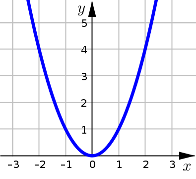
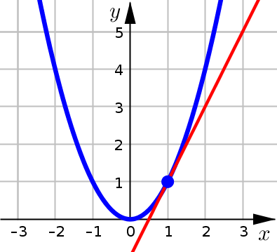
The first thing we need to do is draw (what we think) the tangent line should be at \(x=1\). We use \(x=1\), since we are interested in estimating \(f'(1)\).
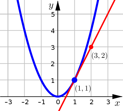
Next we need to estimate the slope of this tangent line by picking two points on the line, and calculating the slope using:
In our graph, we have the point of tangency \(P(1,1)\) and then it looks like \(R\) is a second point on the tangent line with coordinates \((3,2)\). For this second point, its helpful to use one with easily identifiable coordinates. We calculate:
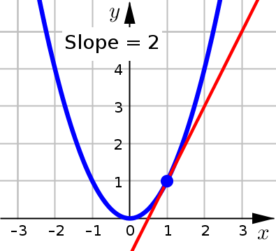
Since we have (our estimate) for the slope of the tangent line, we can conclude:
Slope Forumlas#
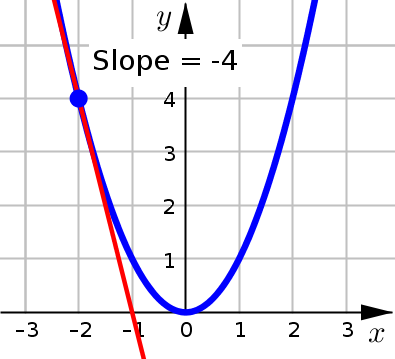
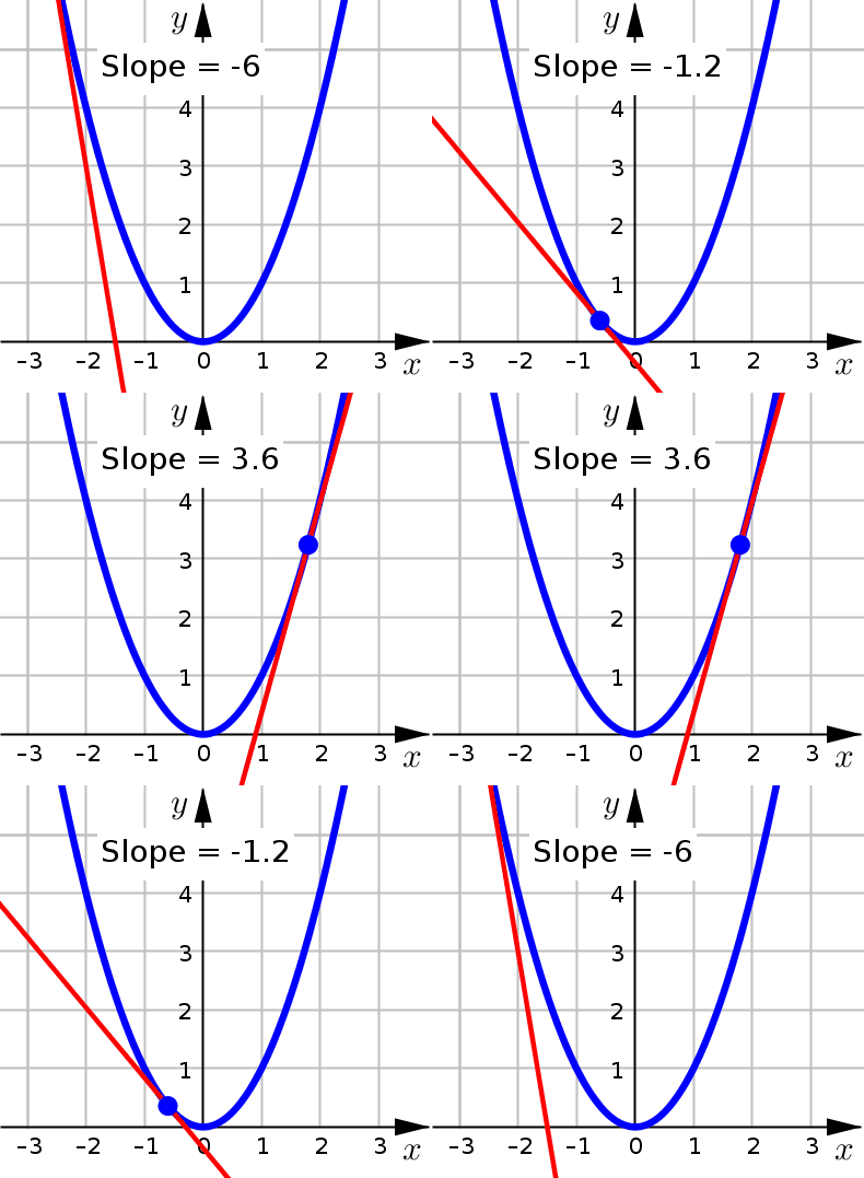
Given any differentiable function, we could repeat this experiment to estimate the slope of the curve at any specific location we want. However we are usually interested in multiple locations, which means we would need to repeat this method over and over again.
It sure would be nice if there was a formula that could just tell us the slope of the graph at any \(x\)-value. There is! This is what the derivative tells us.
Example 1#
The function \(f\), shown in the graph below, gives the population of the United States \(t\) years after the beginning of \(1800\).
What was the average rate of growth of the United States population from \(1840\) to \(1870\)?
How fast was the population growing in \(1840\)?
Was the population growing faster in \(1810\) or \(1860\)?
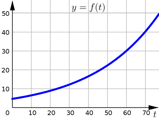
This graph shows the population of the United States (in millions of people) at time \(t\). Where \(t\) represents the number of years after the year \(1800\).
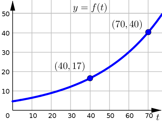
Since \(t\) measures the number of years after \(1800\), in order to find the average rate of growth (change) over the time interval from \(1840\) to \(1870\), we need to use the \(t\)-values \(40\) and \(70\).
To get the average rate of growth, we need to calculate the difference quotient. And to help with this, we look up function values \(f(70)\) and \(f(40)\) using the graph and the corresponding \(y\)-coordinates.
What this value tells us is that from \(1840\) to \(1870\) the population was increasing at an average rate of approximately \(0.77\) million people per year.
(Note that this is approximation, since we really had to estimate the function values in our reading of the graph.)
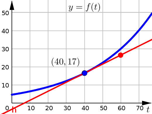
For part (2), we want to find the instantaneous rate of change of \(f\) at time \(t=40\) (year \(1840\)).
We are going to estimate this graphically, by drawing the tangent line to the curve at this point \((40,17)\) and then determining the slope of the line we drew.
Once we have our sketch of the tangent line, we need to pick a second point on this line to use for our slope calculation. It looks like point \((60,27)\) is on the line (try to pick a point that goes through at least one of the grid lines).
Calculating the slope for these two points we get:
This tells us that in the year \(1840\), the population was increasing at a rate of \(0.5\) million people per year.
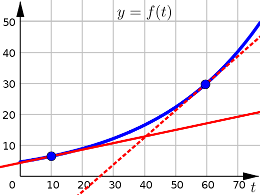
In part (3), we want to use the slope of the graph at \(t=10\) and \(t=60\) to determine if the population was growing faster in \(1810\) versus \(1860\).
We can find the slope of the graph for each of these time values, by drawing in the tangent lines and then estimating the slopes.
However, since we are looking for a comparison, we only need to determine which tangent line has the larger slope (is steeper). Looking at both tangent lines, we see that the one at \(t=60\) is steeper (has a larger positive value). Therefore we can say that the population was growing faster in \(1860\).
