(DC6) Numerical Estimations#
By the end of the lesson you will be able to:
numerically estimate the value of the derivative at a point.
interpret the meaning of a derivative in context and state the units.
Lecture Videos#
Difference Quotient Estimates#
\( \displaystyle \lim_{h\to 0^+} \dfrac{f(a+h)-f(a)}{h} \)
\( \displaystyle \lim_{h\to 0^-} \dfrac{f(a+h)-f(a)}{h} \)
Centered Difference Quotient
Estimating the Derivative Numerically#
In example 2 below, we will demonstrate one technique for approximating derivatives numerically using difference quotients.
Why might we want to estimate a derivative rather than just calculate it exactly? Sometimes (and this is especially true in many applications) we only have a limited amount of information about the function we’re interested in. For instance, in example 2, we only have a table listing a few values of our function - we don’t actually have a nice formula for the function.
Example 2#
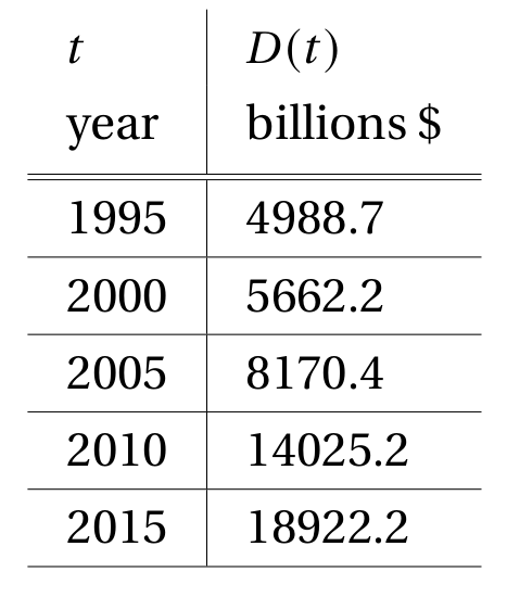
The function \(D\) described in the following table gives the national debt of the United States at time \(t\).
Estimate (and interpret) the value of \(D'(2010)\).
We’re going to start the approximation by calculating a right side difference quotient.
To do this, we’ll calculate the average rate of change of \(D\) over the interval \([2010,2015]\). We use \(t=2010\) because that is the time we want to estimate the derivative at. We then use \(t=2015\) as the other endpoint, because that is the next largest data point on our table. (We use a larger time value because this is a right side difference quotient.)
Next, we’ll calculate a left side difference quotient by looking at the average rate of change of \(D\) over the interval \([2005,2010]\). We use \(t=2010\) again because we want to estimate the derivative at that time. We then use \(t=2005\) as the other endpoint, because that is the next smallest data point on our table. (We use a smaller time value because this is a left side difference quotient.)
Each of the right and left side difference quotients can be used on their own to estimate \(D'(2010)\), but we can improve the approximation by averaging the two together.
We’ve just calculated an approximation for the instantaneous rate of change of \(D\) at time \(t=2010\).
What this value represents, is that in the year \(2010\) the national debt of the United States was increasing at an approximate rate of 1075.18 billions of dollars per year.
We know it was increasing because the value of this derivative is positive. A negative result would have meant that the debt function \(D\) was decreasing in \(2010\).
Units for Rate of Change#
Often when working with functions its helpful to keep track of the units, whether its to perform a dimensional analysis - or just to get a better picture of what’s going on. So you might be wondering: what would be the units for the derivative of a function?
Units
So far we’ve seen a few applied examples in this lesson. What were the dimensions in each of these cases?
Example 1 - Population: Let \(f(t)\) give the population of the U.S. in millions of people \(t\) years after the beginning of \(1800\).
Example 2 - National Debt: Let \(D(t)\) describe the national debt of the United States at year \(t\).
Velocity and Acceleration#
Moving Object: We’ve looked at the problem of motion in a straight line before, and there we saw a function \(s(t)\) describes the position of the object at time \(t\) and function \(v(t)\) describes its velocity. Another important function which we define below is \(a(t)\), the acceleration of the object.
For our discussion here, suppose s(t) describes the height, in meters, of a ball moving in a straight line after \(t\) seconds.
What are the units used to describe its velocity and acceleration?
Instantaneous Velocity
The velocity \(v\) of an object moving in a straight line is:
Acceleration
The acceleration \(a\) of an object moving in a straight line is:

