(IC4) Riemann Sums#
By the end of the lesson you will be able to:
Explain the definition of the definite integral using approximating rectangles.
Calculate a Riemann Sum for a function over a given interval.
Lecture Videos#
Distance Problem#
Estimate the distance traveled by an object during a certain time period (provided the velocity is known at certain times).
Idea: If the velocity remains constant then:
Split up the time period into many small time subintervals.
Assume the velocity is constant on each subinterval.
Approximate the distance traveled in each time subinterval.
Total distance is approximately then the sum of all these subinterval distances.
Example 1#
We want to estimate the distance our car drives during a \(30\)-second time interval. We take speedometer readings every five seconds given by the following table. Use the left endpoints of each subinterval to estimate this distance.
Click through the tabs to see the solution.
Give this a try for yourself first!
Time Subintervals
Based on the table, our time interval is \([0,30]\) and we have effectively split this up into smaller time subintervals all with an equal length of \(5\) seconds.
In order to estimate the total distance traveled over the entire interval, we are going to estimate the distance travled over each subinterval and then sum the results.
Consant Velocity on Each Subinterval
To do this we will assume that we traveled at a constant velocity during each subinterval. For the purposes of this example we will use the initial velocity (left endpoints) as our velocity reading.
This means that throughout:
subinterval \([0,5]\) we will be assuming our velocity was constantly \(v(0)=25\).
subinterval \([5,10]\) we will be assuming our velocity was constantly \(v(5)=31\).
subinterval \([10,15]\) we will be assuming our velocity was constantly \(v(10)=35\).
and so on.
Keep in mind that it would be perfectly valid to use the ending velocity (right endpoints) as our velocity reading for each subinterval.
To calculate the distance traveled during each subinterval, we use the formula:
and the values for velocity and time where:
velocity is the velocity chosen for that subinterval (we’re using initial velocity for our estimate)
time is the length of the subinterval which we usually denote by \(\Delta t\)
For example, to calculate the distance traveled during the first subinterval we get:
The distance traveled during the second subinterval would be:
Repeating this for each subinterval and summing the results, gives us the Total Distance traveled during this entire interval:
Area Problem#
For a given interval, estimate the area under the curve (provided the height of the curve is known at certain locations).
Idea: If the height remains constant then:
Split up the interval into many small subintervals.
Assume the height is constant on each subinterval.
Calculate the area of each approximating rectangle.
Total area is approximately then the sum of the areas of all approximating rectangles.
Example 2#
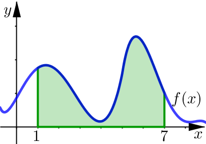
Use the given approximating rectangles to estimate the area under the graph of \(y=f(x)\) on the interval \([1,7]\).
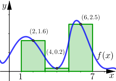
Click through the tabs to see the solution.
Give this a try for yourself first!
Subintervals
The interval is \([1,7]\) and we have effectively split this up into three smaller subintervals all with an equal length of \(2\). In order to estimate the total area under the curve over the entire interval, we are going to estimate the area of each approximating rectangle.
Constant Height on Each Subinterval
To do this we will assume that the height of the curve is constant over each subinterval of the \(x\)-axis. For the purposes of this example we will use the midpoints as our height reading.
This means that throughout:
subinterval \([1,3]\) we will be assuming our curve has a constant height of \(f(2)=1.6\).
subinterval \([3,5]\) we will be assuming our curve has a constant height of \(f(4)=0.2\).
subinterval \([5,7]\) we will be assuming our curve has a constant height of \(f(6)=2.5\).
Keep in mind that it would be perfectly valid to use different points to get the height reading for each subinterval.
To calculate the area under the curve for each subinterval, we use the formula:
and values for Height and Width where:
height is the chosen height for the subinterval (we’re using midpoints for our estimate)
width is the width of the subinterval, which we usually denote by \(\Delta x\)
For example, to calculate the area for the first approximating rectangle we get:
The area of the second approximating rectangle is:
Repeating this for each subinterval and summing the results, gives us an estimate for the Total Area under the curve over this entire interval:
Riemann Sums#
Sigma Notation#
We often use sigma notation to write sums with many terms more compactly. For instance:
\(i\) is an index number and it is usually a positive integer.
\(i=1\) tells us where the index value starts
\(n\) tells us where the index value ends (inclusive)
\(\sum\) tells us to add
Distance and Area Problems#
It turns out that even though the context is different, the calculations we performed in both the distance and area problems were very similar:
What we calculated:
Written in sigma notation:
Here we used \(n=6\) subintervals with:
\(t_i\) values were left endpoints of each subinterval.
\(\Delta t\) is the width of each subinterval.
What we calculated:
Written in sigma notation:
Here we used \(n=3\) subintervals with:
\(x_i\) values were midpoints of each subinterval.
\(\Delta x\) is the width of each subinterval (rectangle).
Riemann Sum#
Essentially the above calculations are so common in many different applications, we give them a special name: Riemann Sums
Riemann Sum
Sample points: \(x_i^*\)-values
Width: \(\Delta x = \dfrac{b-a}{n}\) for interval \([a,b]\) split up into \(n\) subintervals.
Sample Points#
In the above definition we call all of the \(x_i^*\)-values sample points. Essentially these are the numbers we pick from each subinterval. So \(x_1^{*}\) is picked from the 1st subinterval, \(x_2^{*}\) from the 2nd subinterval, and so on. We have full control over what sample points we choose, but some of the more common choices are to use the right endpoints, left endpoints, or midpoints of each subinterval.
This is where we choose each sample point to be the right endpoint of the corresponding subinterval. For interval \([a,b]\) with \(n\) subintervals, the right endpoints can be calculated as:
This is where we choose each sample point to be the left endpoint of the corresponding subinterval. For interval \([a,b]\) with \(n\) subintervals, the left endpoints can be calculated as:
This is where we choose each sample point to be the midpoint of the corresponding subinterval. For interval \([a,b]\) with \(n\) subintervals, the midpoints can be calculated as:
Definite Integral#
Better Estimates#
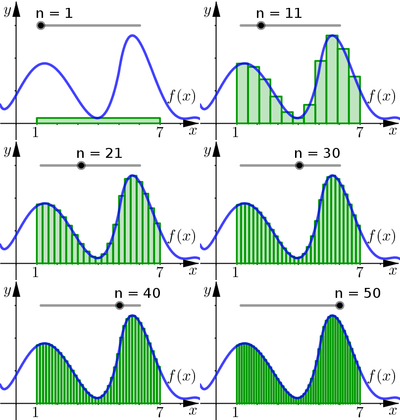
Ultimately, the goal of these Riemann Sums is to get better and better approximates for the area under the curve. How do we do this? Let \(n\) increase.
We see that as \(n\) increases:
We are using more and more approximating rectangles to represent the region, but they are getting thinner and thinner.
The result here is that the approximating rectangles better represent the region under the graph.
So we expect that our area calculations will be a better approximation as well.

The area of these rectangles is given by the following Riemann Sum.
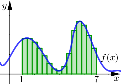
The area of these rectangles is given by the following Riemann Sum.
Definition#
Definite Integral
Let \(f\) be a function defined for \(a\leq x \leq b\). The definite integral of \(f\) from \(a\) to \(b\) is:
provided this limit exists and gives the same value for all possible sample points. If it does exist, we say that \(f\) is integrable on \([a,b]\).
Notation:
We call \(\Delta x = \dfrac{b-a}{n}\) the width of each subinterval.
\(n\) represents the number of subintervals.
\(x_i\) are the sample points (usually right, left, or midpoints)
What Functions are Integrable?#
Integrable Functions
If \(f\) is continuous on \([a,b]\), or if \(f\) has only a finite number of jump discontinuities, then \(f\) is integrable on \([a,b]\). That is, the definite integral exists:
Issue: While not every function can be integrated, this theorem tells us that we can integrate all functions that are either:
continuous on \([a,b]\)
continuous on \([a,b]\) except for a finite number of jump discontinuities.
How to Calculate: Calculating a definite integral directly from this limit definition is usually a non-trivial (difficult) task. It technically is possible, but it is usually quite a bit of work. Instead we have already seen the preferred way to calculate definite integrals: the Fundamental Theorem of Calculus.
Example 3#
Express the following limit as an integral on the interval \([0,\pi]\).
Solution (Click to see answer and explanation)
We can think of the limit and sigma combining to form the integral sign. (In fact, the integral sign is an elongated letter “s”.)
On the other side of the expression, during the limit process the \(\Delta x\) term becomes the differential \(dx\). In fact, you can think of the differential as denoting the infinitesimal width of a subinterval.
Example 4#
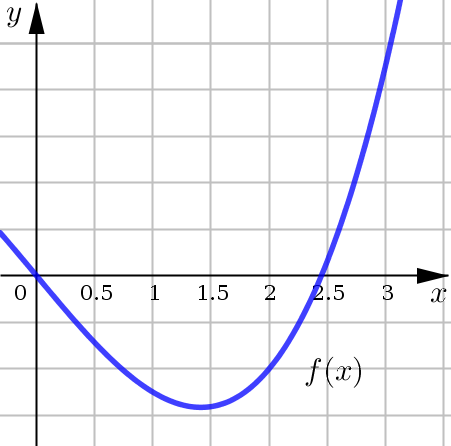
Evaluate the Riemann Sum for \(f\), taking the sample points to be right endpoints and \(n=6\) where:
In order to calculate this Riemann Sum, the first thing we need to calculate is the width of the subintervals:
Since our interval is \([a,b]=[0,3]\) and the directions specifically indicated that we should use \(n=6\).
Next, we need to find the right endpoints for each subinterval. The start by finding the first right endpoint using the formula \(x_1^* =a+\Delta x\), and then progressively add \(\Delta x\) to get the next endpoint.
We can then use these right endpoints to draw in our approximating rectangles.
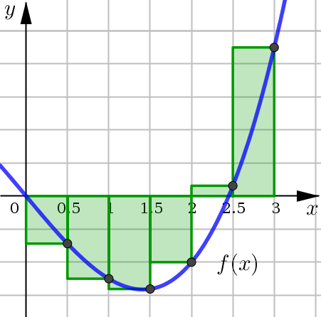
Finally, we use these right endpoints and \(\Delta x\) to calculate the Riemann Sum:
Since we have the right endpoint Riemann Sum with \(n=6\), we sometimes denote this approximation using the notation \(R_6\). (Similar notation for \(L_6\) and \(M_6\).)
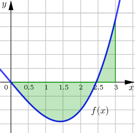
Notice that in our approximation, the negative function values correspond to the approximating rectangles which are below the horizontal axis. And the positive function values correspond to those rectanges which are above.
This is why we normally interpret the definite integral as representing the Net Area.

Let’s look at these Riemann Sums from example 4 a little bit further, just to investigate what the limit process looks like.

The net area of these rectangles is given by the following Riemann Sum.
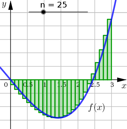
The net area of these rectangles is given by the following Riemann Sum.

