(DC2) Instantaneous Velocity

(DC2) Instantaneous Velocity#

By the end of the lesson you will be able to:

find the average velocity on a time interval and the instantaneous velocity at a specified time.

Lecture Videos#

Introduction to Velocity#

Position Function#

The Position Function

The position function is a function \(s(t)\) that denotes the position of an object moving in a straight line at time \(t\).

For example:

Car driving on a straight road.
Object dropped from a cliff.

Static

Animation

Observation

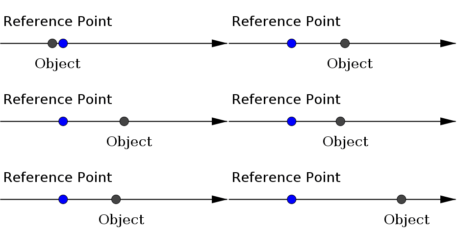
In the animation, notice that the object:

starts off moving towards the right
slows down and temporarily stops
moves to the left
slows down and stops again
and then starts moving back towards the right.

And as you watch this, you can tell when the object is moving fast versus when it’s moving slow.

Average Velocity#

When we think of a moving object, one of the first natural questions to ask is:

How fast is it moving?

We have an intuitive understanding that a moving object has a specific velocity at each instant of time. Think about when you’re driving a car, you can look down, read the speedometer, and see the speed you’re traveling, at any time. But how do we actually measure this?

Well, a few examples of the units we use to measure velocity are \(m/s\) or \(ft/s\) (meters per second or feet per second). What these units imply is that we are actually looking at how far we travel during a specific interval of time. For example: we traveled 5 meters east in 1 second.

The idea of measuring the change in our position relative to the change in time is where we start, we call this the average velocity. For an object with position function \(s(t)\) we have:

\[ \text{average velocity} = \dfrac{\text{displacement}}{\text{time elapsed}} = \dfrac{s(b)-s(a)}{b-a} \]

where:

\(a=\) starting time
\(s(a)=\) starting position
\(b=\) ending time
\(s(b)=\) ending position

Note that these values are comparatively easy to measure for an actual moving object. We have the tools to measure the start and stop time, as well as the starting and ending position.

Instantaneous Velocity#

Instantaneous Velocity

The velocity \(v(a)\) at time \(t=a\) of an object moving in a straight line is:

\[ v(a)=\lim_{h\to 0 }\dfrac{s(a+h)-s(a)}{h} \]

Where does this formula come from?

Let’s start with our average velocity over time interval \([a,b]\). Letting \(b\to a\), we are essentially calculating the average velocity over smaller and smaller time intervals. As these time intervals shrink, the average velocity gets closer and closer to the instantaneous velocity at time \(t=a\).

\[ v(a)= \lim_{b\to a} \left[ \text{Average Velocity} \atop \text{during } [a,b] \right] = \lim_{b\to a} \dfrac{s(b)-s(a)}{b-a} \]

Usually, it is helpful to rephrase these variables in terms of a time interval. Let’s use \(h\) to represent the length of the time interval, then \(h=b-a\). We could then rewrite the limit in terms of this new variable \(h\), noting that:

if \(h=b-a\), then \(b=a+h\)
and as \(b\to a\) the time interval is getting smaller and smaller which means \(h\to 0\)

Substituting these in, we get the equation stated above:

\[ v(a) = \lim_{b\to a} \dfrac{s(b)-s(a)}{b-a} = \lim_{h\to 0} \dfrac{s(a+h)-s(a)}{h} \]

Example 3#

Suppose that a rock is dropped from a height of \(50m\) with position function \(s(t)=4.9t^2\).